Markers #

last modified February 24, 2026

~8 minute read

Markers are the symbols we use to show the location of a value in our data visualization. Most commonly, they are encountered in scatterplots, but one might also consider the bars of a bar chart or Sankey diagram to be markers as well. Here, we are going to focus mostly on the types of markers found in scatterplots, but will touch on bars at the end.

Establishing Contrast in Markers #

The primary objective when selecting markers is determining how to achieve appropriate contrast between distinct data groups. If we understand this visual mechanism, we can intentionally calibrate how similar or different data series appear. Naturally, if we keep all parameters identical, we lack contrast and lose the ability to differentiate between series. Consider a plot charting the increasing cost of tuition for two BIG10 Universities, mapped exclusively with identical filled circles:


In the figure above, we have failed to distinguish the two universities visually; therefore, it is impossible to determine if their tuition trajectories intersect (e.g., around 2014). There are specific storytelling instances where this ambiguity might be intentional—for instance, if the core narrative focuses strictly on overarching macro-trends where highlighting individual schools would create unnecessary distraction. However, in most analytical scenarios, the viewer requires the ability to tell distinct series apart. The central design question then becomes, “Exactly how different do we want them to appear?” This is a parameter we can precisely control by modulating the following spatial and color properties.

Orientation #

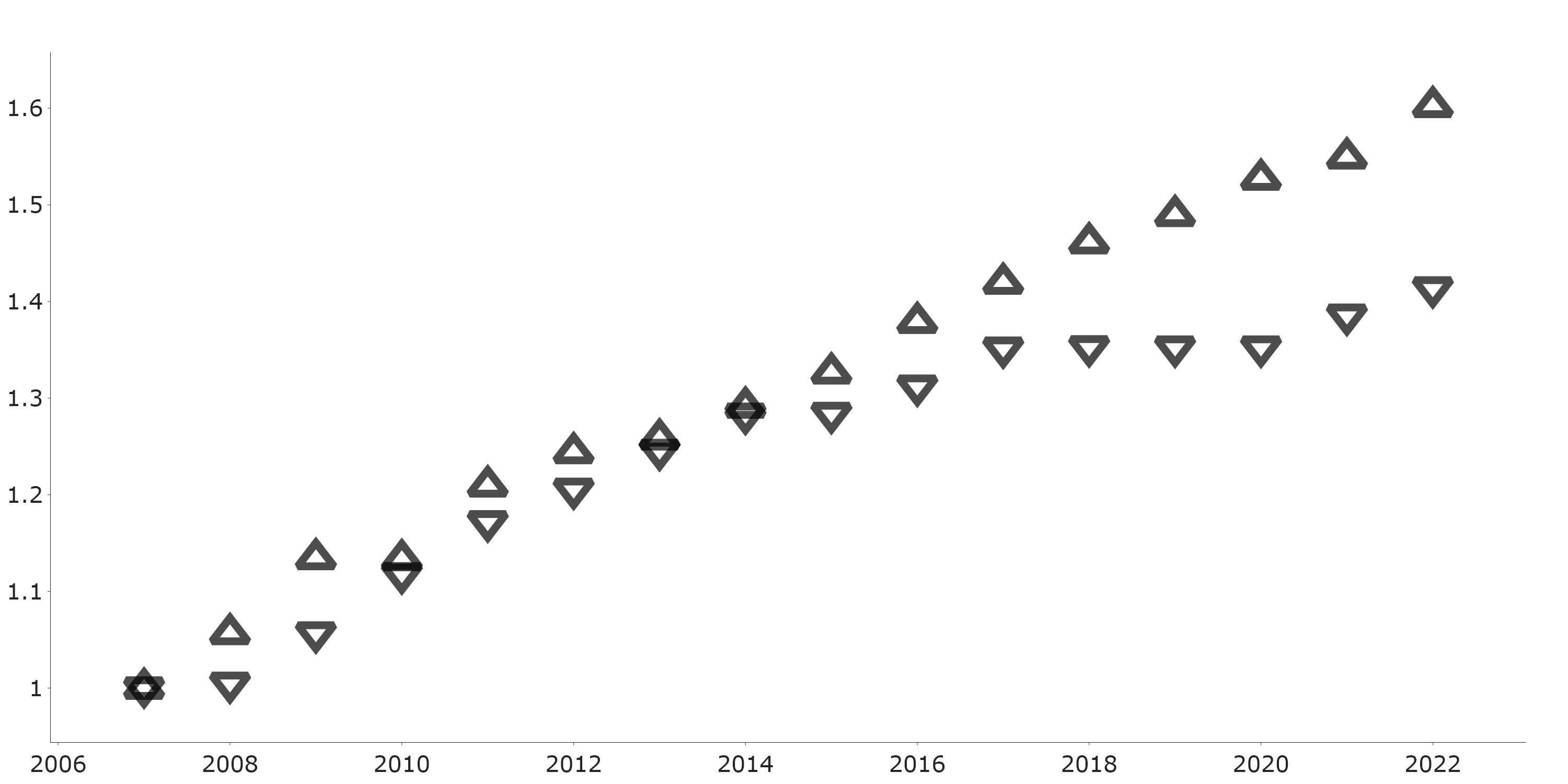
With orientation, we are talking about taking the exact same shape and rotating it. For instance, we might use up and down triangles:

Or we might use squares and diamonds:

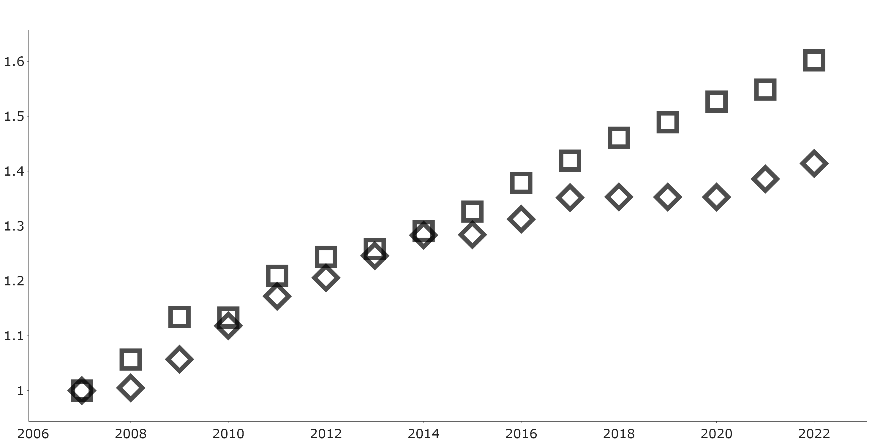
One thing that is clear is that we can tell these shapes apart. However, as we will see below, the contrast between these shapes is rather subtle. So, these are changes that are good to choose, if the distinction between the plots is not the main point, but we still want people to be able to follow individual trends, should they wish to.

Outline #

Another way to create subtle contrast is to change the outline on a shape:

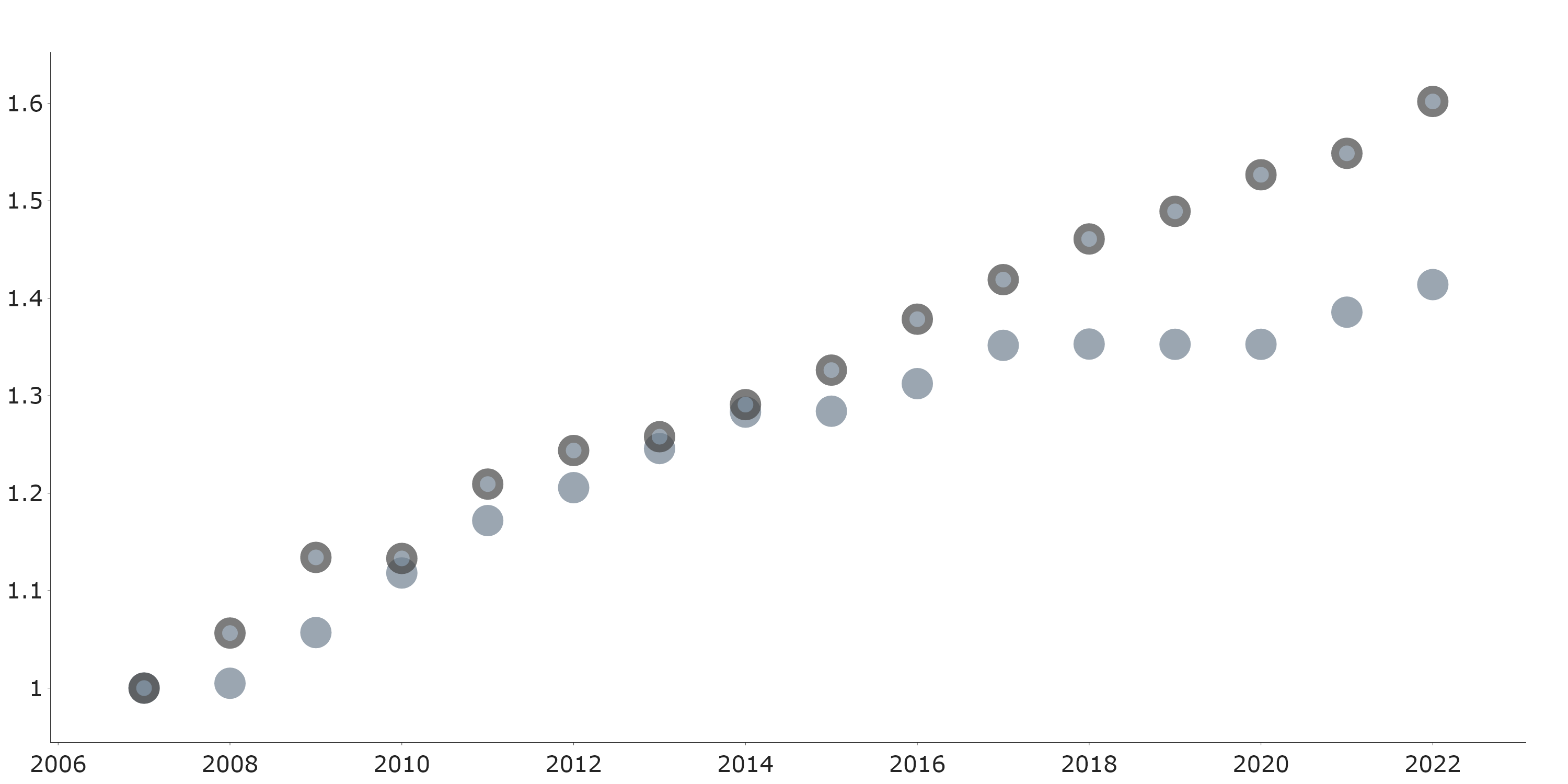
Here, we have simply added an outline to one of the shapes, while maintaining the overall size. One can tell the two apart, though, again you probably have to focus a bit on the graph to do so.

Fill #

Yet more contrast can be realized by using filled versus non-filled shapes:

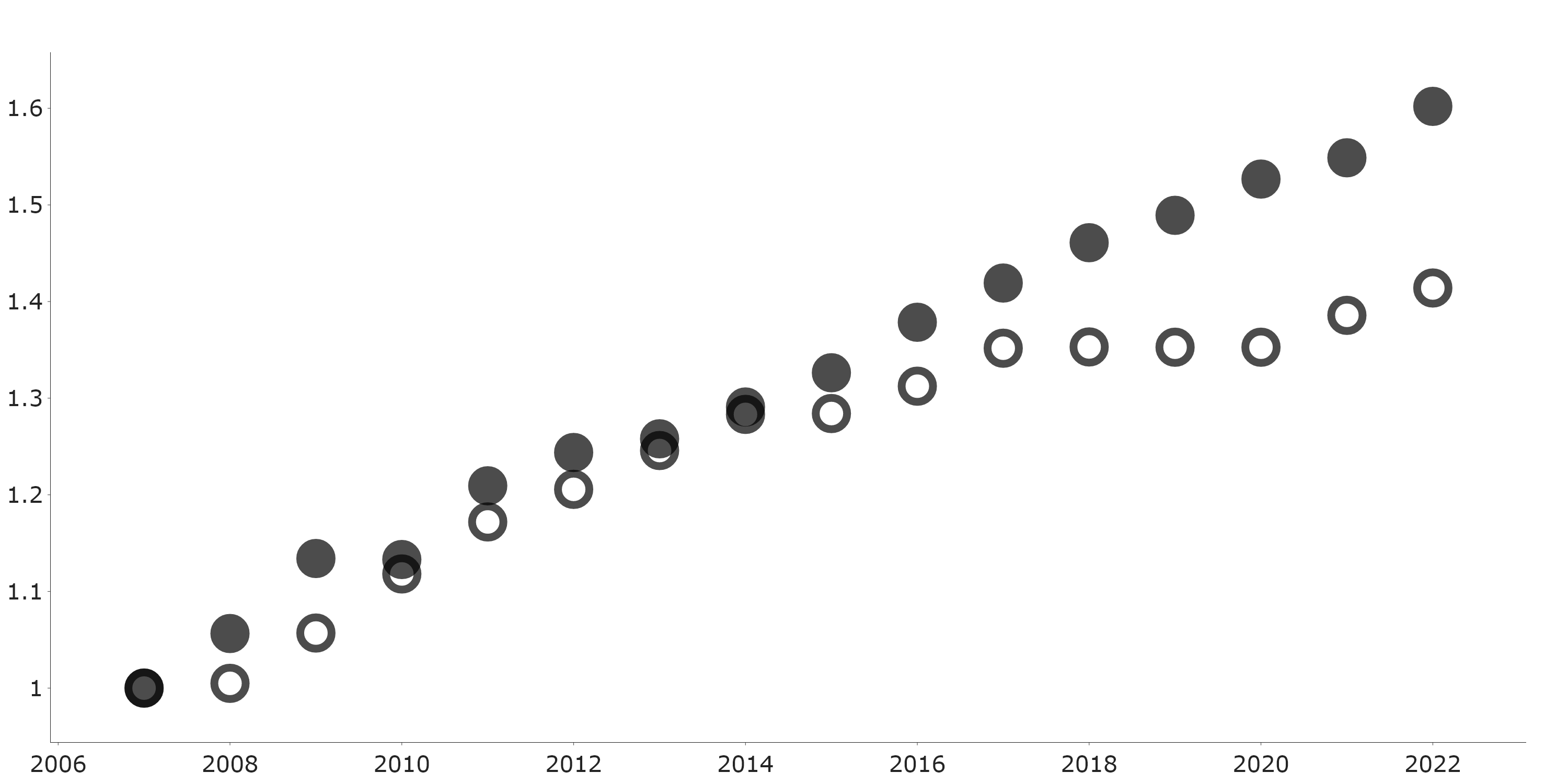
Where the shapes here only differ in if there is a fill to the shape.

To my eye, this is the first change that leads to a plot where the difference is obvious. That is, I no long really have to focus on the plot to determine the overall trends for each data series. But, because the shapes are the same, they still do blur together a bit when they converge. If you are ok with this effect, then changes in the presence or absence of fill can be a great choice.

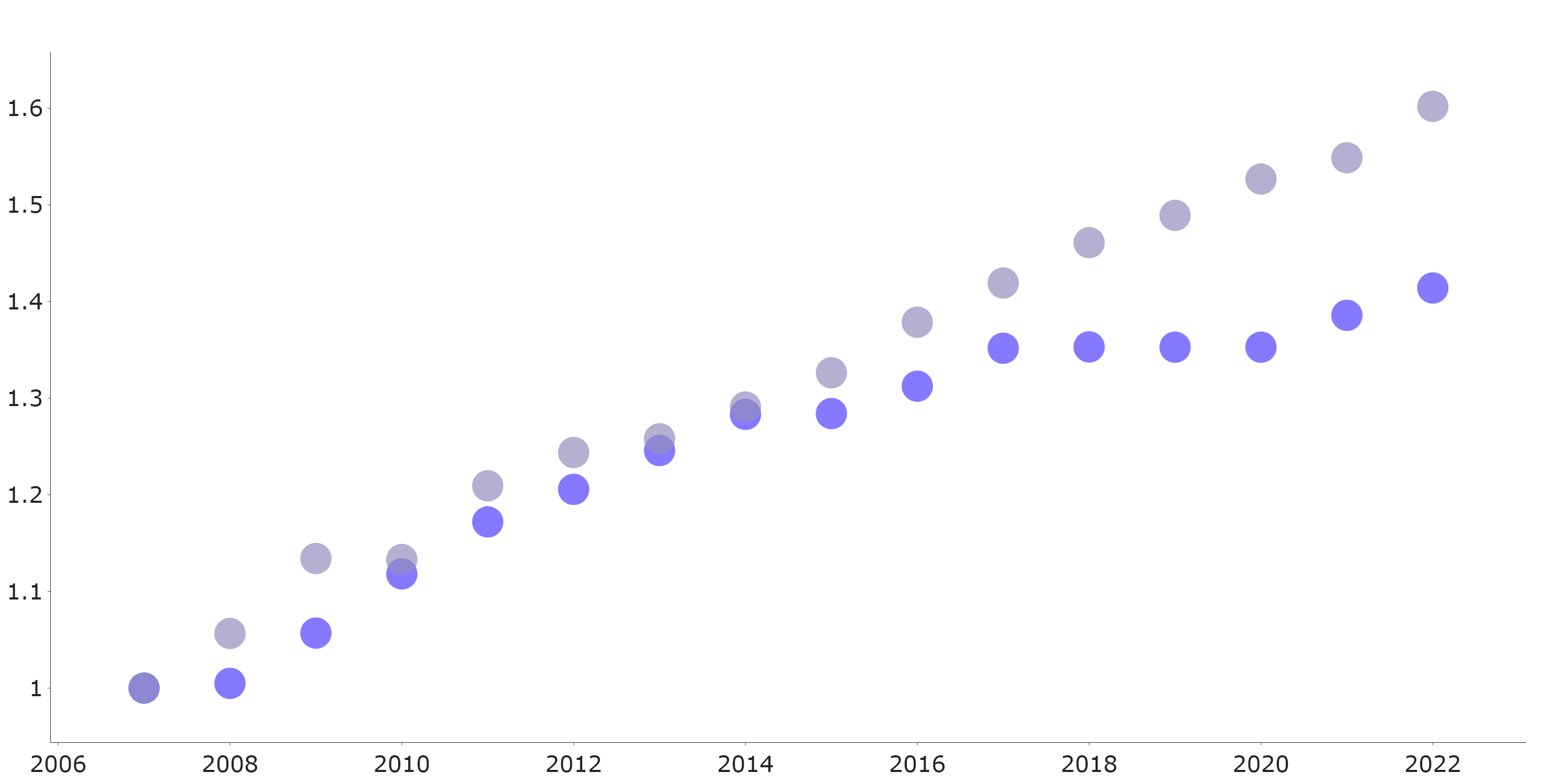
Size #

To me, changing the size of the markers can have the same contrast as changes in fill:

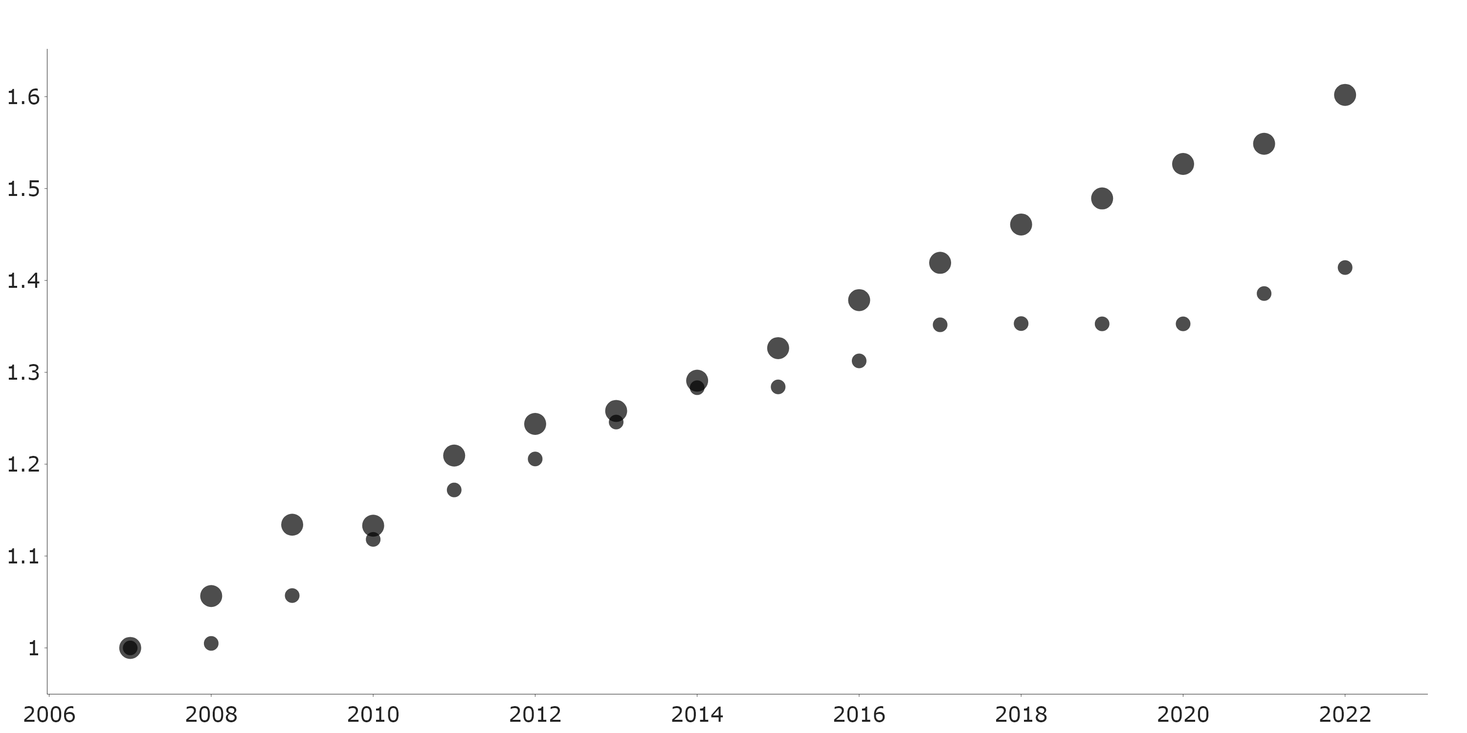
Where the differences in size make it quite apparent that there are two series and which is which.

Similar to changes in fill, however, the series blend together whenever they converge. Additionally, the change in size will have the effect of emphasizing one series over the other. Thus, I would use changes in size only when you are trying to make this emphasis. Otherwise, I would use any of the other parameters discussed here.

Shape #

While manipulating orientation yields relatively subtle contrast, shifting the physical geometry of the shape itself generates much stronger differentiation. Here, we illustrate the transition from a circle to a square:

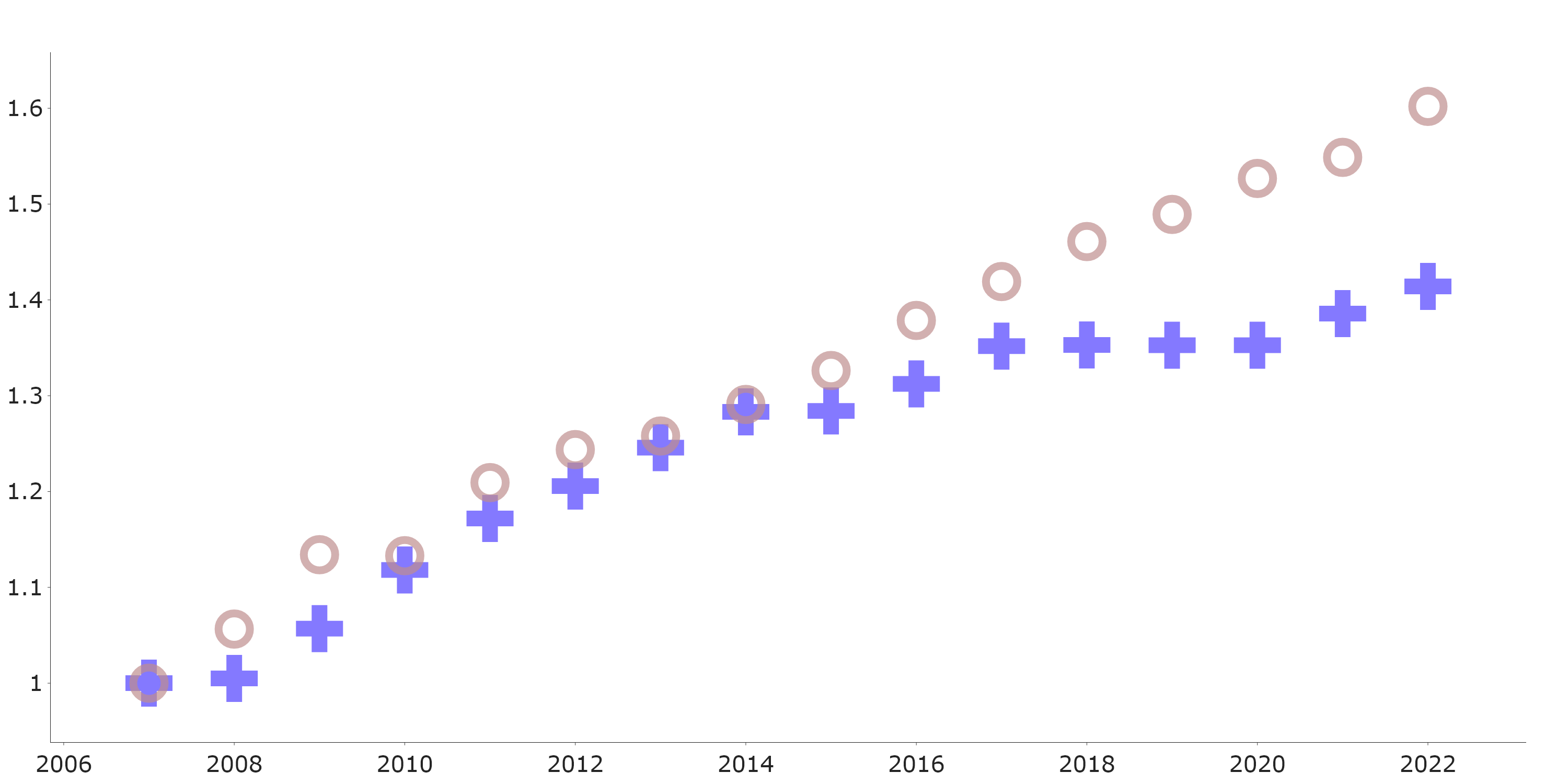
Alternatively, we might transition from circles to prominent plus marks:

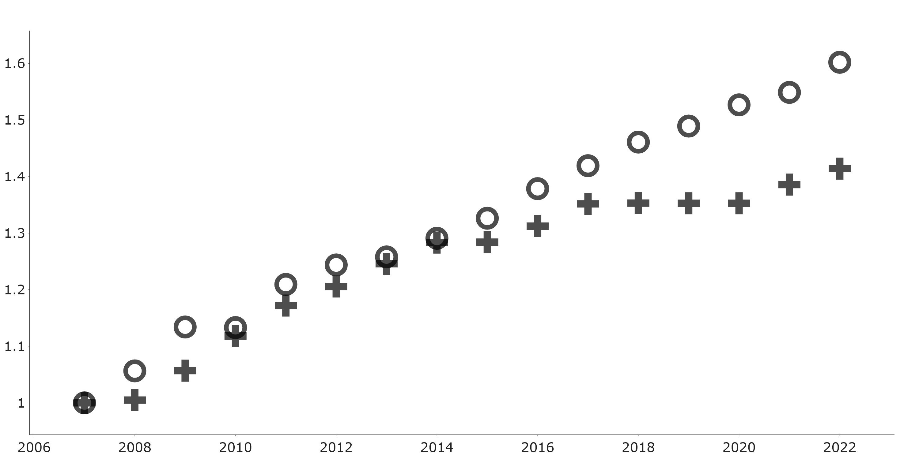
While numerous geometric shapes exist, maximum categorical contrast is generally achieved by pairing shapes with fundamentally opposed structural properties—such as juxtaposing smooth, rounded forms against sharp, angular ones.

Color #

When considering color, we noted that it is useful to think about color in terms of hue, saturation, and value, and so we can consider differences in each of these channels.

Hue #

In general, hue is a very nice variable to attain contrast in markers. The strongest contrast for most people will be attained with complimentary color:

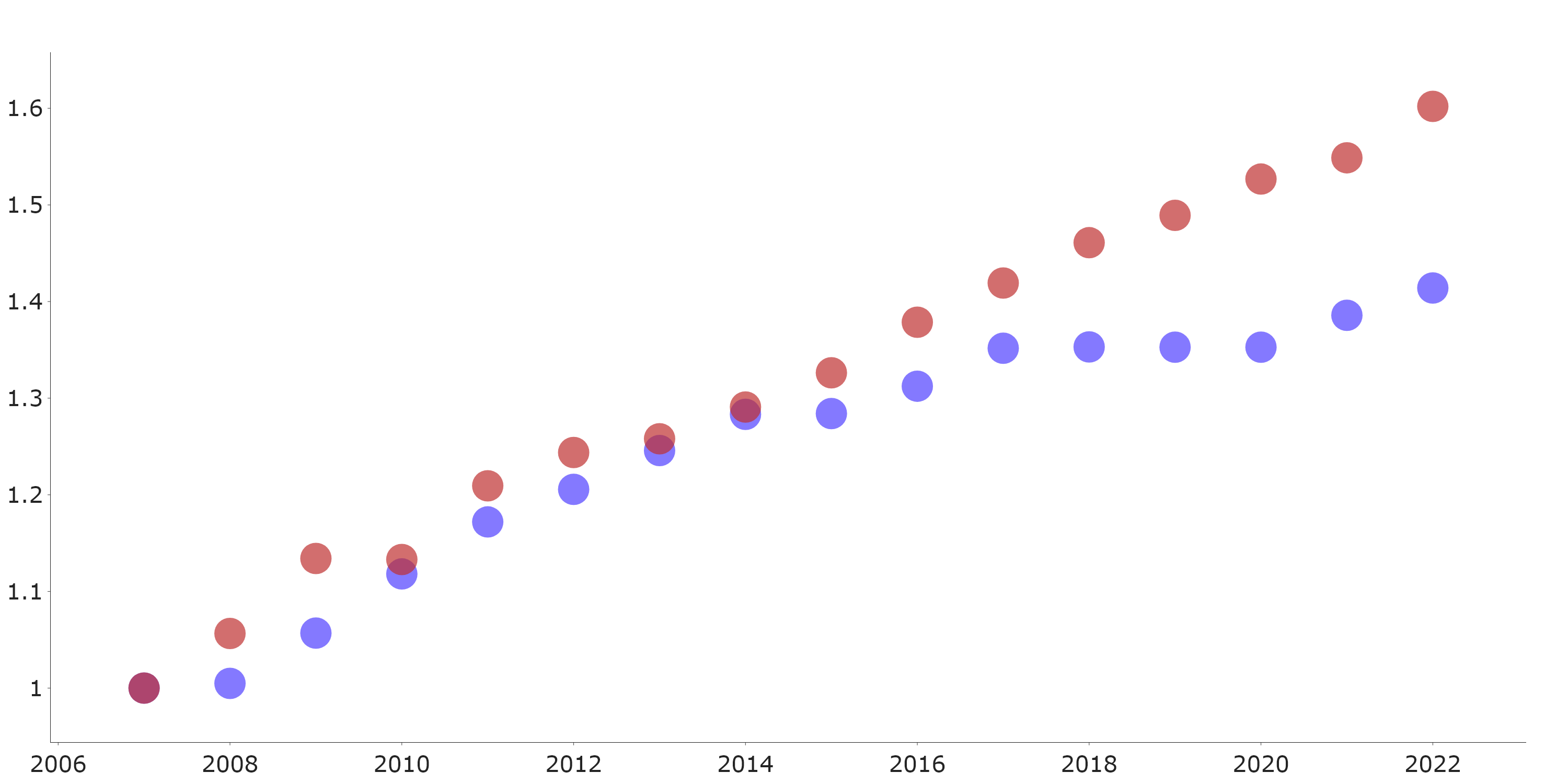
This plot has colors with 75% saturation and 75% value, but different hues. Though in the page on color we said that most color information comes from value, hue still works well here, because we are not trying to assign a quantitative value based on color. If we were, then value would be the clear choice. But hue allows us to readily differential between series, based on category.

Value #

Of course, value does produce good contrast between series:

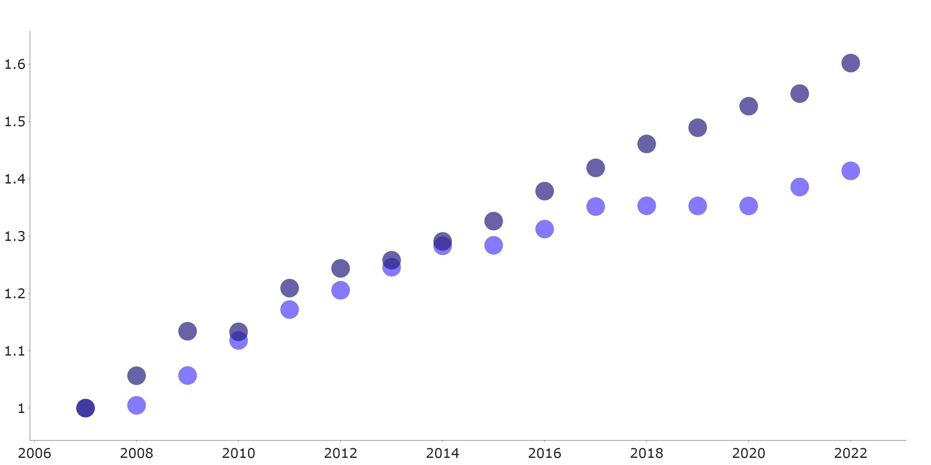
The series in this plot are both the same hue and both have 75% saturation, but the brighter one has 100% value while the the other has 50% value. Differences in value is something to consider using if we want to have a plot with analogous colors, or even a monochrome color scheme (as used above). So, don’t feel like you need to turn to hue, if you don’t want to.

Saturation #

Saturation is probably the weakest channel for realizing contrast, though it is still effective:

In this plot, the two series are the same hue, both with 75% value, but one has 100% saturation while the other has 50% saturation. You can use saturation when you don’t want a change in hue or value, and you want the shapes to look the same, but you still want to try to realize contrast between markers.

Combining differences #

Of course, one needn’t use any of the above marker parameters in isolation. Instead, they can be combined in order to create even higher contrast, here is a plot that uses difference in shape, saturation, value, and hue, all together to create very strong contrast.

Limitations #

One thing that is important to realize is that the contrast that is obtained between markers is dependent on the size of the markers. Above, we saw a very high contrast pair of markers, but if we were to make the markers too small, we will loose most (if not all) of this contrast.

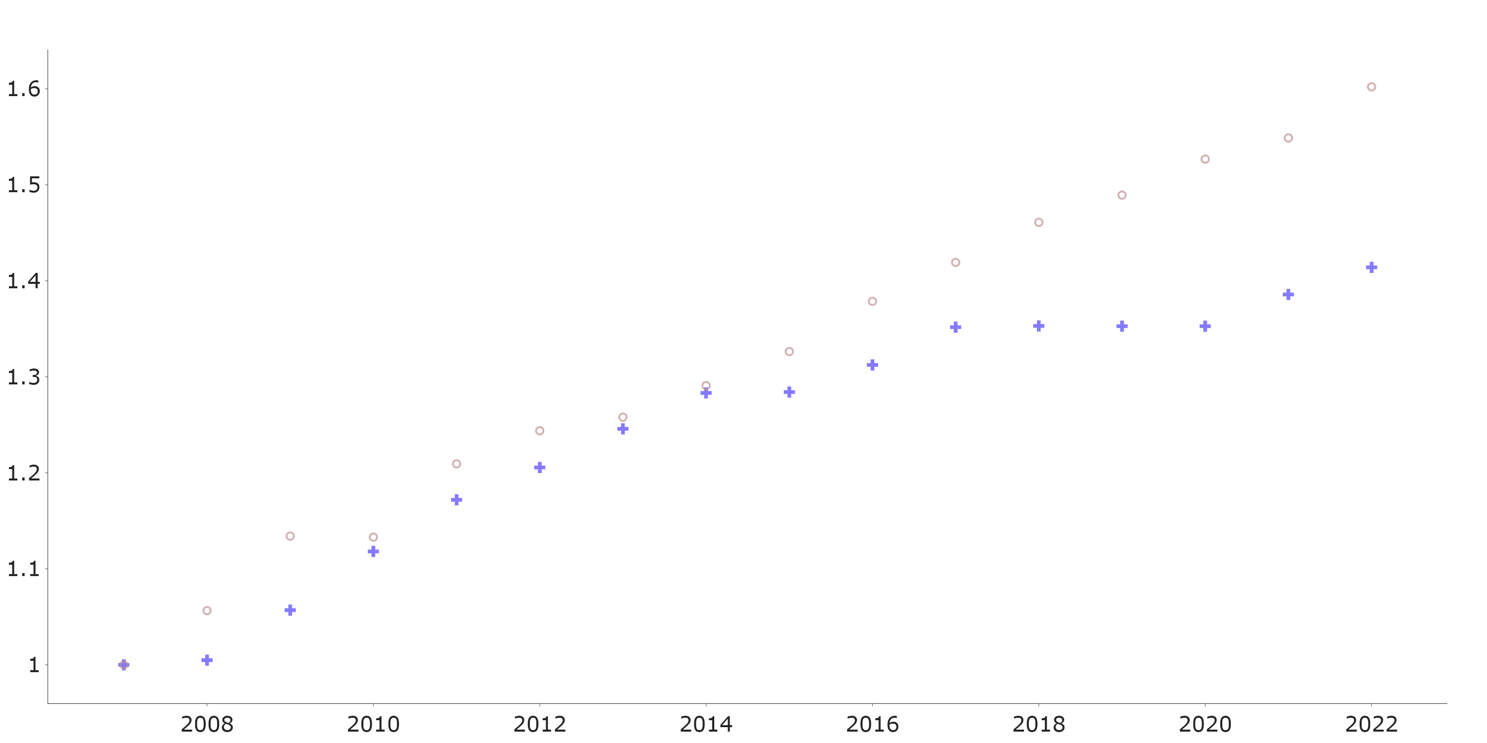
Here we see that, perhaps the only contrast that remains is between the value. So, really make sure you are plotting things at a size that allows for contrast to be realized.

Other considerations #

One last point to consider, when talking about markers is that the shape of the marker can have unexpected effects on the appearance of the data. For instance, if you choose a shape that is asymmetric along the vertical axis, then when you have closely spaced points, you will have a strange appearance of the data. For instance, consider the following plot:

Here, the top plot utilizes triangles as discrete markers. Because the base of the triangle is flat while the apex is sharp, closely layered sequential markers inadvertently create the perceptual illusion of a solid, jagged line segment forming along the top.

In the bottom plot, pentagons are employed, producing an even more distorting optical illusion where overlapping dark markers appear to double back, implying the data is traveling in reverse along the x-axis.

The essential takeaway is to critically evaluate not only how shapes generate contrast against each other, but how the geometric properties of a chosen shape might unconsciously distort the perception of the continuous data trend. As a general rule, prioritizing highly symmetric symbols (both vertically and horizontally) minimizes these unintended optical artifacts.

Bars #

Many of the things we have considered above could be used when we are considering contrast between bars… for instance, in a bar chart. Of course, we don’t have access to all of these options, as we will rarely (if ever) be changing the shape or bars, or the orientation of individual bars. Additionally, since the size of the bars is the means by which we encode the quantitative values, we should not think of size as a means to control contrast. But the fact remains that we can change the outline, fill, and color of the bars. These can lead to contrast, just as in markers.

Where, again to my eye, I like the changes in color best, without outlines, but you can, of course, make your own design choices.

Key takeaways #

There is really no mystery about attaining contrast in markers. You simply make a list of the parameters that you can change, and then go about trying to change them. If there are any surprises here, it is that changes in orientation can have a surprisingly subtle effect and that one needs to consider the size of markers carefully. However, the first is really a tool in disguise—a way to create subtle contrast when desired—while the latter is a general consideration in all of graphic design.

And, as ever, a golden rule of design applies: the quality of your choices can only be judged in the final creation. That is, just because your ideas for contrast make sense in theory, you should always evaluate the final product and decide if you are attaining the results you want.

page last modified February 24, 2026